Random Binary Alloy

The idea behind this model is to study disorder. We’ll look at a 1D chain of sites, with the usual nearest neighbor hopping. The Hamiltonian looks like

\[H = \sum_i \epsilon_i + V \sum_i c^\dagger_i c_{i+1} +h.c\]

where

\[\epsilon_i = \begin{cases} \epsilon_a & p\\ \epsilon_b & (1-p) \end{cases}\]

In other words, we choose between the energy \(\epsilon_a\) with a probability \(p\).

Making the Hamiltonian

Our overall goal is to analyze the wave functions generated from the eigenvalue equation

\[H|\psi\rangle = E|\psi\rangle\]

i.e. the time-independent Schrödinger equation.

The Method

To construct the Hamiltonian we’ll use a method known as exact diagonalization, where we explicitly construct a matrix representation of a finite sized system. After obtaining the matrix, we can diagonalize it exactly to obtain the full spectrum with np.eigh and analyze the wave function properties.

Note: using np.eigh vs np.eig is very important as there’s better convergence once the eigenvalues are restricted to be real

Neat! While ED generally takes place in the \(S_z\) spin basis (where each element the Hamiltonian acts on is a configuration of spins), this model can instead be diagonalized in the site basis. What this means practically is that we can get to a bigger system size than if we used the spin basis and we don’t have to interpret the many-body basis - we directly calculate natural orbitals.

The Code

def makeH(L,eps_a,eps_b,V,p=None,plotDisorder=False):
    if p is None:
        p=0.5
    #make the Hamiltonian 
    H = np.zeros([L,L])
    for site in range(L):
        #periodic boundary conditions are on
        H[site,(site+1)%L] = -V
        H[(site+1)%L,site] = -V
    # to obtain the on site energy
    # we'll make a random vector of 1s and 0s,
    # with a probability of p for 1
    # then the diagonal will be
    # eps_b*(1,...1) + (eps_a-eps_b)*(random vector)
    diag = eps_b*np.ones([L])
    diag += (eps_a-eps_b)*np.random.choice([0, 1], size=(L,), p=[p,1-p])
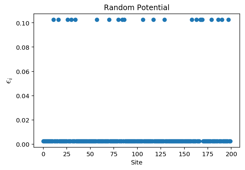
    if plotDisorder:
        print("The disordered system looks like:")
        plt.plot(diag,'o')
        plt.xlabel("Site")
        plt.ylabel(r"$\epsilon_i$",fontsize=15)
        plt.title("Random Potential")
        plt.show()
    H[np.diag_indices_from(H)] = diag
    return H

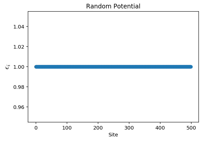
Case 1: Zero Disorder

\(p=0\), which is the same as having a disorder strength of 0. We’ll look at 3 states with the lowest, middle, and highest energy.

eps_a = 1
eps_b = 1
V = 1
L = 500
H1 = makeH(L,eps_a,eps_b,V,p=0,plotDisorder=True)
plt.subplot(121)
plt.imshow(H1)
plt.title("Hamiltonian matrix")
plt.colorbar()
plt.subplot(122)
E1,v1 = np.linalg.eigh(H1)
plt.plot(E1)
plt.title("Eigenvalue spectrum")
plt.tight_layout()
plt.show()


offsets = [0,L//2,-3]
names= ["Low","Middle","High"]
fig, axes = plt.subplots(3,3, sharex=True,sharey=True,figsize=(10.0, 10.0))
for start in range(len(offsets)):
    for i in range(3):
        axes[start,i].plot(v1[:,offsets[start]+i],'o-')
        if i==1:
            axes[start,i].set_title(names[start])
axes[len(offsets)//2,0].set_ylabel(r"$|\psi_i\rangle$",fontsize=15)
axes[-1,1].set_xlabel("Site Label",fontsize=15)
axes[0,0].set_title("Ground State")
plt.show()

The disordered system looks like:

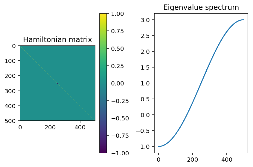
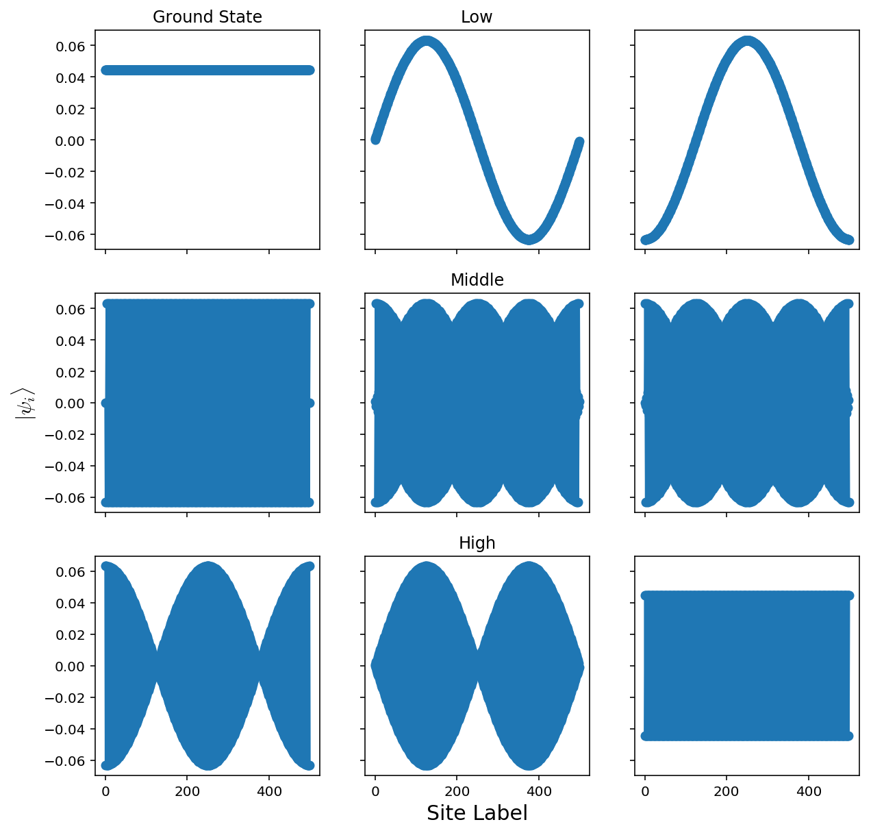
Here, the states we get are extended throughout the system. This is because we have 0 disorder! The analytic solution to this is to diagonalize through a Fourier transform, where we get a dispersion of \(E(k)=\epsilon-2V\cos(k)\)

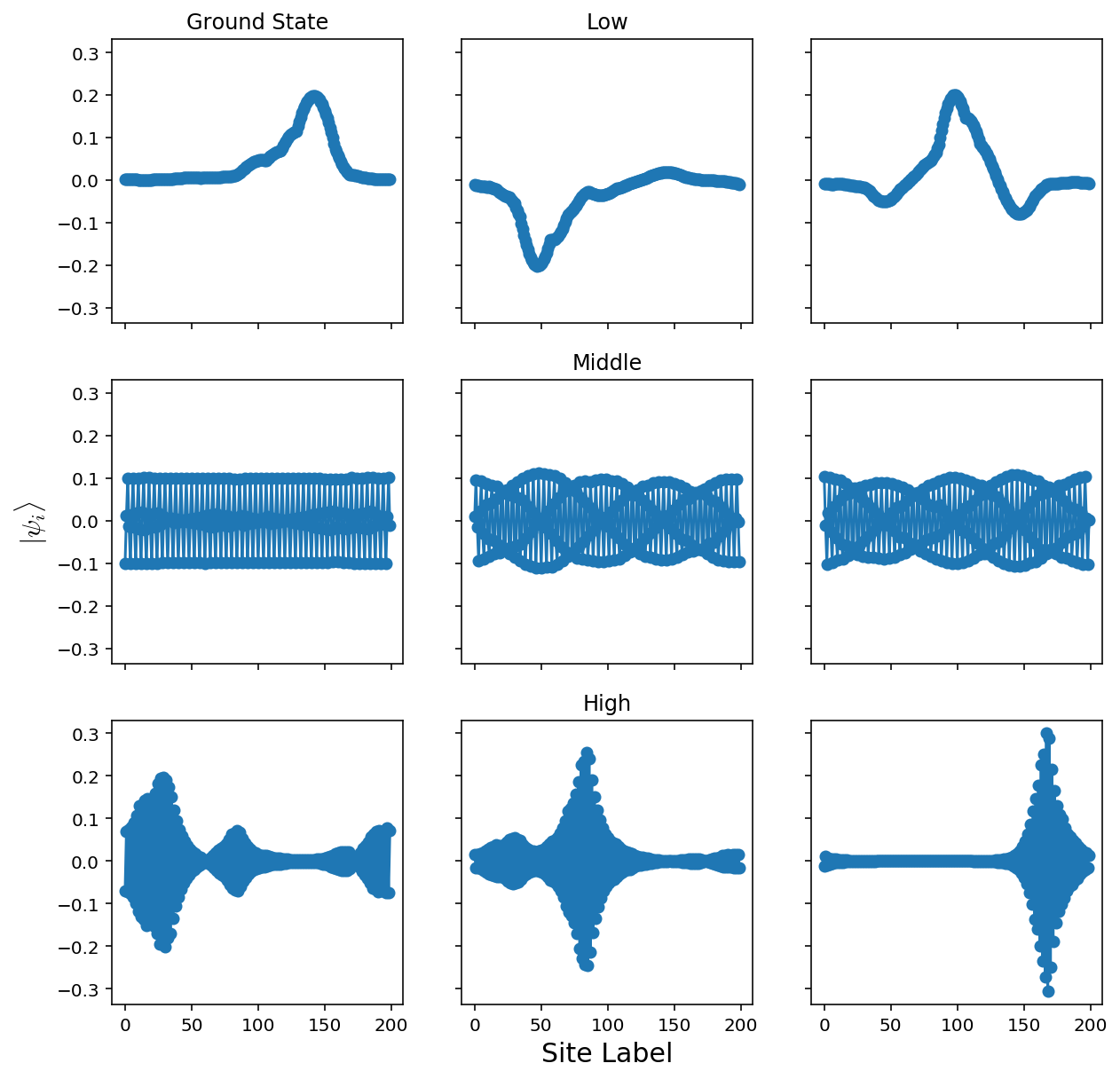
Case 2: High Disorder

\(\Delta\epsilon=V/4, p=0.5\)

eps_a = V/4
eps_b = V/2
V = 1
L = 200
H1 = makeH(L,eps_a,eps_b,V,plotDisorder=True)
E1,v1 = np.linalg.eigh(H1)
plt.plot(E1)
plt.title("Eigenvalue spectrum")
plt.show()

offsets = [0,L//2,-3]
names= ["Low","Middle","High"]
fig, axes = plt.subplots(3,3, sharex=True,sharey=True,figsize=(10.0, 10.0))
for start in range(len(offsets)):
    for i in range(3):
        axes[start,i].plot(v1[:,offsets[start]+i],'o-')
        if i==1:
            axes[start,i].set_title(names[start])
axes[len(offsets)//2,0].set_ylabel(r"$|\psi_i\rangle$",fontsize=15)
axes[-1,1].set_xlabel("Site Label",fontsize=15)
axes[0,0].set_title("Ground State")
plt.show()

The disordered system looks like:

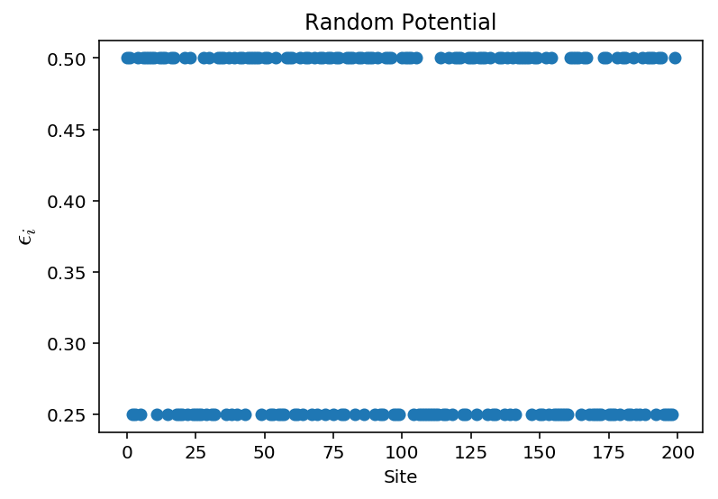
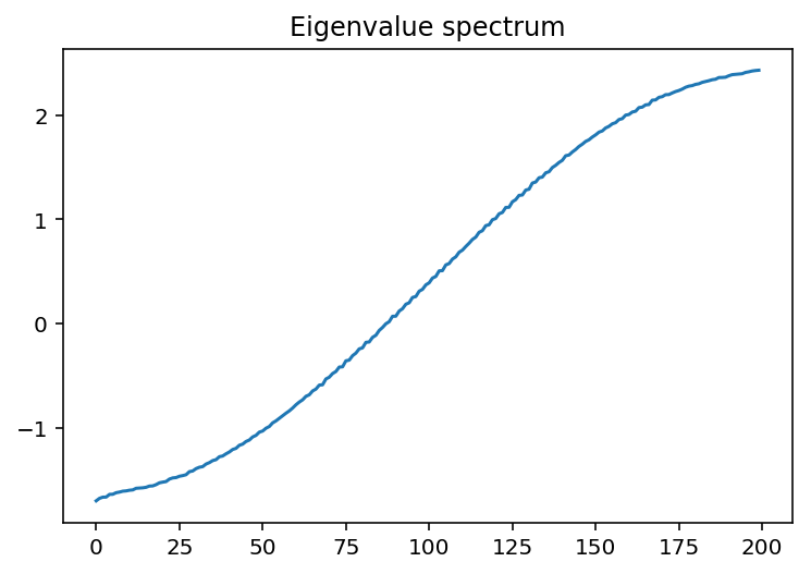
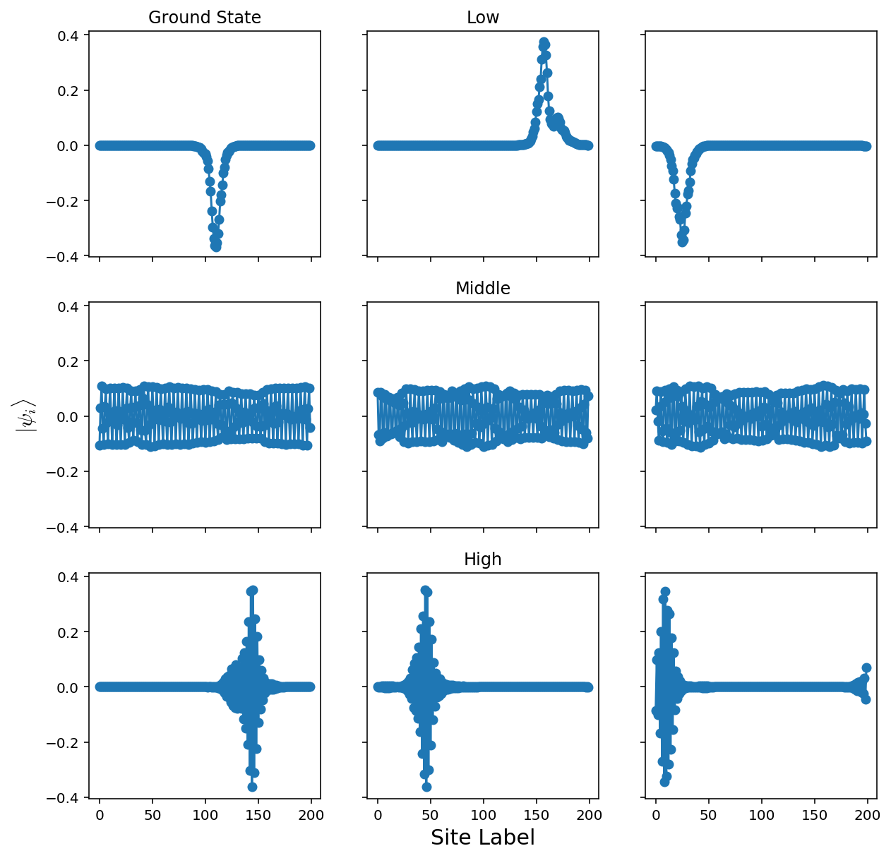
That’s more like it! The lowest energy states are localized - this is the fact that they decay exponentially away from some localized area. These correspond to the places where the random potential is the “least random.”

Case 3: Low Disorder

\(\Delta\epsilon=V/4, p=0.1\)

eps_a = 0.01*V/4
eps_b = eps_a+0.1
p=0.1
V = 1
L = 200
H1 = makeH(L,eps_a,eps_b,V,p,plotDisorder=True)
E1,v1 = np.linalg.eigh(H1)
plt.plot(E1)
plt.title("Eigenvalue spectrum")
plt.show()

offsets = [0,L//2,-3]
names= ["Low","Middle","High"]
fig, axes = plt.subplots(3,3, sharex=True,sharey=True,figsize=(10.0, 10.0))
for start in range(len(offsets)):
    for i in range(3):
        axes[start,i].plot(v1[:,offsets[start]+i],'o-')
        if i==1:
            axes[start,i].set_title(names[start])
axes[len(offsets)//2,0].set_ylabel(r"$|\psi_i\rangle$",fontsize=15)
axes[-1,1].set_xlabel("Site Label",fontsize=15)
axes[0,0].set_title("Ground State")
plt.show()

The disordered system looks like:

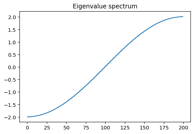
When we lower the disorder strength, the localization spreads. We can try and get a picture of this by plotting several ground states for various disorder strengths

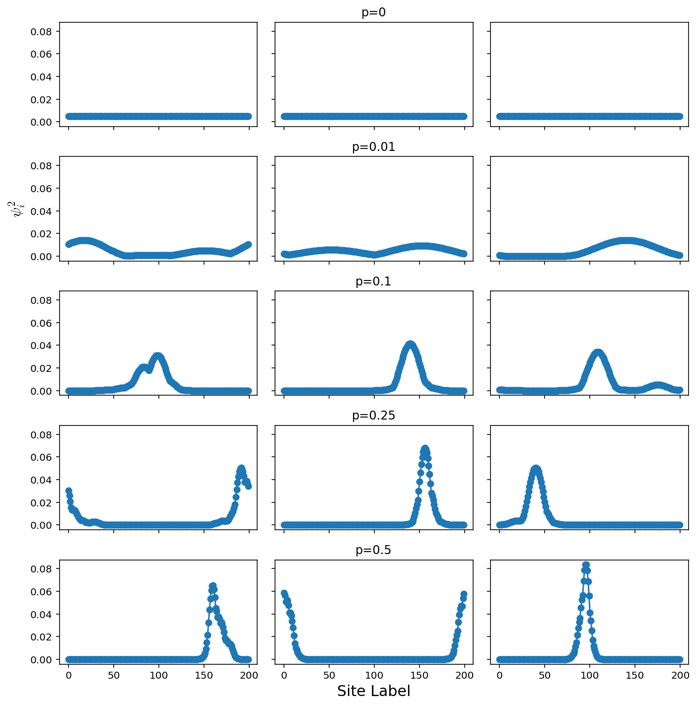
Comparison of Disorder Strengths

Constant ∆ε, variable probability

eps_a = V/4
eps_b = eps_a+0.1
V = 1
L = 200
tries = 3
pList = [0,0.01,0.1,0.25,0.5]
fig, axes = plt.subplots(len(pList),tries, sharex=True,sharey=True,figsize=(10.0, 10.0))
for p in range(len(pList)):
    for i in range(tries):
        H1 = makeH(L,eps_a,eps_b,V,pList[p],plotDisorder=False)
        E1,v1 = np.linalg.eigh(H1)
        axes[p,i].plot(np.abs(v1[:,0])**2,'o-')
    axes[p,tries//2].set_title("p="+str(pList[p]))
axes[len(offsets)//2,0].set_ylabel(r"$\psi_i^2$",fontsize=15)
axes[-1,1].set_xlabel("Site Label",fontsize=15)
plt.tight_layout()
plt.show()

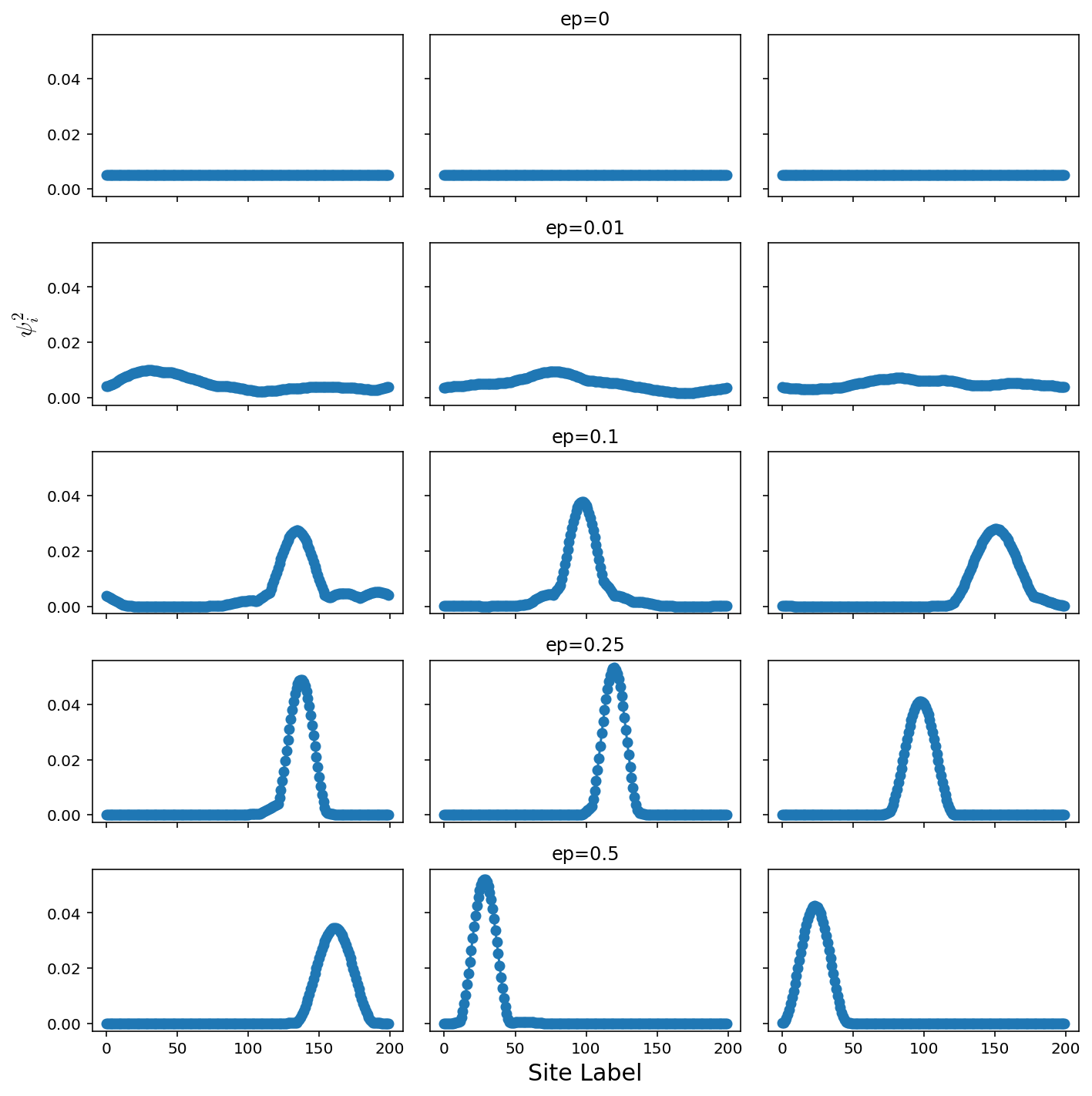
Constant probability, variable energy difference

eps_a = V/4
p=0.1
V = 1
L = 200
tries = 3
epList = [0,0.01,0.1,0.25,0.5]
fig, axes = plt.subplots(len(pList),tries, sharex=True,sharey=True,figsize=(10.0, 10.0))
for ep in range(len(epList)):
    for i in range(tries):
        H1 = makeH(L,eps_a,eps_a+epList[ep],V,p,plotDisorder=False)
        E1,v1 = np.linalg.eigh(H1)
        axes[ep,i].plot(np.abs(v1[:,0])**2,'o-')
    axes[ep,tries//2].set_title("ep="+str(epList[ep]))
axes[len(offsets)//2,0].set_ylabel(r"$\psi_i^2$",fontsize=15)
axes[-1,1].set_xlabel("Site Label",fontsize=15)
plt.tight_layout()
plt.show()

#===============================================
%load_ext watermark
%watermark

2018-02-05T09:20:40-06:00

CPython 3.6.3 IPython 6.2.1

compiler : GCC 4.2.1 Compatible Apple LLVM 9.0.0 (clang-900.0.37)
system : Darwin
release : 16.7.0
machine : x86_64
processor : i386
CPU cores : 4
interpreter: 64bit