
Exact Diagonalization for the 1D Heisenberg Chain
The Heisenberg model is given by \(H = -\sum_{\langle i,j \rangle}J_{ij}(S_i \cdot S_j)\) We choose nearest neighbors to get
\[\begin{align} H =& -\sum_{\langle i \rangle}J_{i,i+1}(S_i \cdot S_{i+1}) \\ =&-\sum_{\langle i \rangle} J_{z} S^z_i S^z_{i+1} + \frac{J_{xy}}{2}(S^+_i S^-_{i+1} + S^-_i S^+_{i+1})) \\ \end{align}\]We choose a lattice of length \(L\) and lattice spacing \(\Delta\). It is also possible to create a magnetic field (more on why later), using a new term \(H_B = -h \sum_i S_z\)
Overview
This will be an overly inefficient, but clear, way to generate the Hamiltonian for exact diagonalization. The steps we’ll take:
- Generate the basis
- this involves finding all binary numbers with the same number of high bits, as this Hamiltonian respects \(S_z\) symmetry
- Generate the Hamiltonian in Matrix form
- For each state in the basis, apply \(H|\psi\rangle\) and record the values/connections
- This will involve a diagonal term and off diagonal term
- put them in the appropriate spot in a (dense) matrix
- Solve for the matrix’s eigenvalues and eigenvectors
- put everything together for a nice package!
- Analyze the output
Note: A more efficient way of doing this would be to use sparse matrices, but our \(S_z\) block is small enough to not have memory constraints
Code
Helper Functions
These are some nify functions that help with visualization and debugging
import numpy as np
import matplotlib.pyplot as plt
import scipy.stats as spst
def basisVisualizer(L,psi):
    '''Given psi=(#)_10, outputs the state in arrows'''
    #ex: |↓|↑↓|↑|↑|
    psi_2 = bin(psi)[2:]
    N  = len(psi_2)
    up = (L-N)*'0'+psi_2
    configStr = "|"
    uparrow   = '\u2191'
    downarrow = '\u2193'
    for i in range(L):
        blank = True
        if up[i] == '1':
            configStr+=uparrow
            blank = False
        if up[i] == '0':
            configStr+=downarrow
            blank = False
        if blank:
            configStr+="_"
        configStr +="|"
    print(configStr)
def countBits(x):
    '''Counts number of 1s in bin(n)'''
    #From Hacker's Delight, p. 66
    x = x - ((x >> 1) & 0x55555555)
    x = (x & 0x33333333) + ((x >> 2) & 0x33333333)
    x = (x + (x >> 4)) & 0x0F0F0F0F
    x = x + (x >> 8)
    x = x + (x >> 16)
    return x & 0x0000003F
#helper function to print binary numbers
def binp(num, length=4):
    '''print a binary number without python 0b and appropriate number of zeros'''
    return format(num, '#0{}b'.format(length + 2))[2:]
1. Generate the basis
Because there are a lot of states we’ll need to consider in a given hilbert space, we must be as concise as possible when writing a representation down. Because the computer already uses binary numbers, we’ll take advantage of binary operations and write all states as a binary number. An example of this is below
Convention
a state will have up spins as 1 and down spins as 0 since we don’t have double occupency Here is an example of |↑|↑|↓|
print("The binary number for |up up down> is: ",int('110',2))
print("In binary the state is:",binp(int('110',2),3))
print("The state",int('110',2),"can be visualized as:")
#use helper function to visualize
basisVisualizer(L=3,psi=int('110',2))
The binary number for |up up down> is:  6
In binary the state is: 110
The state 6 can be visualized as:
|↑|↑|↓|
we now create a function that will return a list of lists, where each internal list contains all the appropriate binary numbers with a given $S_z$ configuration
def makeSzBasis(L):
    basisSzList = [[] for i in range(0,2*L+1,2)] #S_z can range from -L to L, index that way as well
    #this is probably a bad way to do it
    # count bits is O(log(n)) and loop is O(2**L) :(
    for i in range(2**L):
        Szi = 2*countBits(i) - L
        basisSzList[(Szi+L)//2].append(i)
    print("L =",L,"basis size:",2**L)
    return basisSzList
Let’s take a look at the distribution of hilbert space, specifically $S_z$
for L in [7,10]:
    basisSzList = makeSzBasis(L)
    SziVals  = []
    sizeVals = []
    for i in range(len(basisSzList)):
        SziVals.append(-L+2*i)
        sizeVals.append(len(basisSzList[i]))
    plt.bar(SziVals,sizeVals,label="L="+str(L))

plt.xlabel(r"$S_z$",fontsize=15)
plt.ylabel("# of elements",fontsize=15)
plt.legend()
plt.show()
L = 7 basis size: 128
L = 10 basis size: 1024
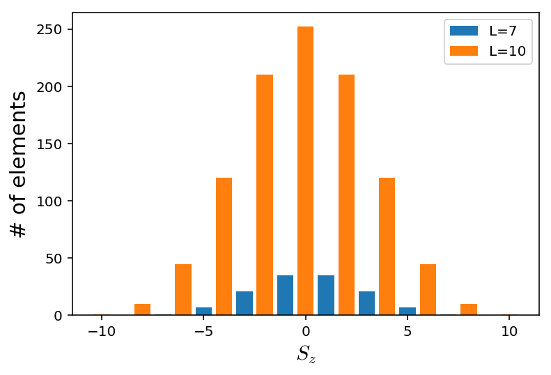
As expected, we see there are more ways to make \(S_z=0\) than anything else, and the distribution looks normal in behaivor. The problem with exact diagonalization is as we increase system size, there are exponentially more states we need to keep track of
2. Generate the Hamiltonian
To create a dense matrix of the Hamiltonian we’ll need two things. A lookup table that converts an element of the hilbert space (like 6) to its index in the Hamiltonan matrix. Then we’ll also need something that takes each state and spits out all the states its connected to, and the values of this connection. This is added into the Hamiltonian matrix. Here, I’ve hard coded it in but more general techniques for both can be used
def makeH(SzList,L,Jxy,Jz,h):
    '''Make a 1D Heisenberg chain of length L with Jxy,Jz and magnetic field h out of an SzList of states'''

    basisMap = {}
    stateID  = 0
    #generate an ordering
    for state in SzList:
        #print(state) #basisVisualizer(L,state)
        basisMap[state] = stateID
        stateID+=1
    nH = stateID
    H = np.zeros([nH,nH])
    #now fill H
    for state in SzList:
        idxA = basisMap[state]
        H[idxA,idxA] += -h*countBits(state) # B field
        for i in range(L):
            j = (i+1)%L #nearest neighbors are hard coded here
            if (state>>i & 1) == (state>>j & 1):#matching bit check
                H[idxA,idxA] += -Jz/4
            else:
                H[idxA,idxA] -= -Jz/4
                mask = 2**(i)+2**j
                stateB= state^mask #this flips the bits at i,j
                idxB = basisMap[stateB]
                H[idxA,idxB]+= -Jxy/2
    #print(np.all(H==H.T)) #check if Hermitian and is coded properly; very slow
    return H
3. Solve for the eigenvalues and eigenvectors
After making \(H\) for each block in \(S_z\), we’ll record all the energies and where the ground state is
def getSpectrum(L,Jxy,Jz,h):
    '''Returns lowestEnergy,
               Sz sector of the GS,
               GS eigenvector,
               and all energies'''
    basisSzList  = makeSzBasis(L)
    energies     = []
    lowestEnergy = 1e10

    for Szi,SzList in enumerate(basisSzList):
        #print('=============')
        #print("Sz sector:",-L+2*Szi)
        #print('=============')
        H     = makeH(SzList,L,Jxy,Jz,h)
        lam,v = np.linalg.eigh(H)
        energies.append(lam)
        #keep track of GS
        if min(lam) < lowestEnergy:
            lowestEnergy  = min(lam)
            GSSector      = -L+2*Szi
            GSEigenvector = v[:,lam.argmin()]

    print("Energies assembled!")
    print("Lowest energy:",lowestEnergy)
    print("The ground state occured in Sz=",GSSector)
    return (lowestEnergy,GSSector,GSEigenvector,energies)
lowestEnergy,GSSector,GSEigenvector,energies=getSpectrum(4,-1,-1,0)
for i in energies:
    print(i)
L = 4 basis size: 16
Energies assembled!
Lowest energy: -1.9999999999999996
The ground state occured in Sz= 0
[1.]
[-1.00000000e+00 -2.25514052e-17  0.00000000e+00  1.00000000e+00]
[-2.00000000e+00 -1.00000000e+00 -6.19908411e-17  0.00000000e+00
  6.84227766e-49  1.00000000e+00]
[-1.00000000e+00 -2.25514052e-17  0.00000000e+00  1.00000000e+00]
[1.]
Plotting routines:
def generatePlots(L,Jxy,Jz,h):
    (lowestEnergy,GSSector,
     GSEigenvector,energies) = getSpectrum(L,Jxy,Jz,h)
    total_energies = [en for szlist in energies for en in szlist]
    maxE           = np.max(total_energies)
    offset = 0
    for i in range(len(energies)):
        plt.plot(range(offset,len(energies[i])+offset),energies[i],'o')
        offset+=len(energies[i])
        if len(energies)-4>i>2:
            if i%2==0:
                plt.text(offset-200,maxE+1,"Sz="+str(-L+2*i))
            else:
                plt.text(offset-200,maxE+0.5,"Sz="+str(-L+2*i))

    plt.xlabel("Arbitrary Order",fontsize=15)
    plt.ylim([lowestEnergy-0.5,maxE+2])
    plt.ylabel("Energy",fontsize=15)
    plt.title(r"XXZ model with $L="+str(L)+",\,\,\, J_z="+str(Jz)+",\,\,\, J_{xy}="+str(Jxy)+"$",fontsize=15)
    plt.plot([0,offset],[lowestEnergy,lowestEnergy],'--',label="Ground State")
    plt.legend(loc='lower right')
    plt.show()
    print('====')
    plt.plot(GSEigenvector,'o-')
    plt.xlabel("state order",fontsize=15)
    plt.ylabel(r"$|\psi_0\rangle$",fontsize=15)
    plt.title("Ground State Eigenvector \nwith $L="+str(L)+",\,\,\, J_z="+str(Jz)+",\,\,\, J_{xy}="+str(Jxy)+"$",fontsize=15)
    plt.show()

    basisSzList   = makeSzBasis(L)
    GSEigenvector = np.abs(np.round(GSEigenvector,10)) #rounding errors
    bigStatesID   = np.argwhere(np.abs(GSEigenvector) == np.max((GSEigenvector))).reshape((1,-1))

    #Get the states
    print("The biggest states are:")
    for state in bigStatesID[0]:
        bigStates = basisSzList[(GSSector+L)//2][state]
        basisVisualizer(L,bigStates)
4. Physics
We’ll look at two systems, an antiferromagnet and a ferromagnet
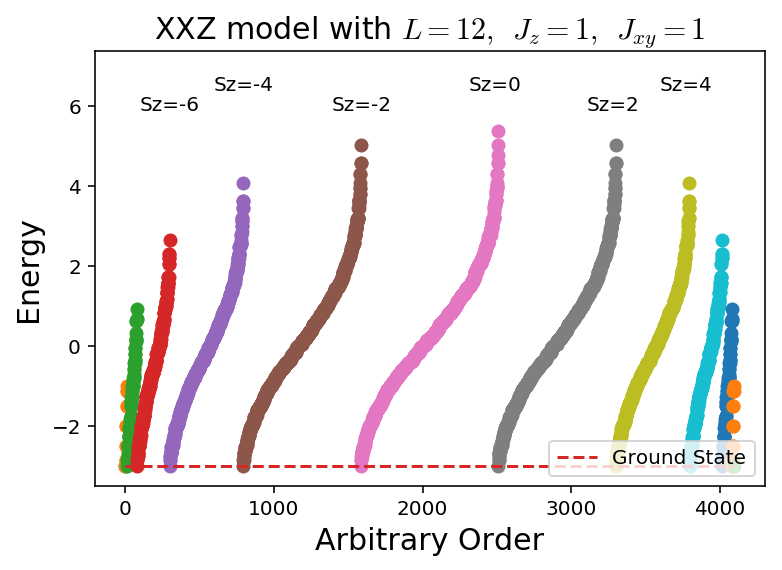
Ferromagnet
#Constants of the problem
L   = 12
Jxy = 1     # when J<0 it is antiferromagnetic
Jz  = 1     # J_z = J_xy = J is the normal Heisenberg model instead of XXZ model
h   = -1e-5 # small h field to break degeneracy
generatePlots(L,Jxy,Jz,h)
L = 12 basis size: 4096
Energies assembled!
Lowest energy: -3.0
The ground state occured in Sz= -12
====
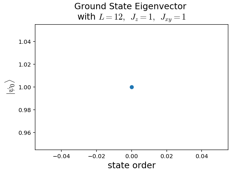
L = 12 basis size: 4096
The biggest states are:
|↓|↓|↓|↓|↓|↓|↓|↓|↓|↓|↓|↓|
Ground State Eigenvector
This is exactly the maximal ferromagnetic state! We added the tiny magnetic field so that we could easily choose the up one over the down one, something that would naturally happen in nature but is hard to get on the computer. There are also degenerate product states in every \(S_z\) sector that are now gapped by the magnetic field.
Antiferromagnet
All we have to do is swap the sign on \(J_z,J_{xy}\)
%%time
#Constants of the problem
L   = 12
Jxy = -1
Jz  = -1
h   = 0
generatePlots(L,Jxy,Jz,h)
L = 12 basis size: 4096
Energies assembled!
Lowest energy: -5.387390917445205
The ground state occured in Sz= 0
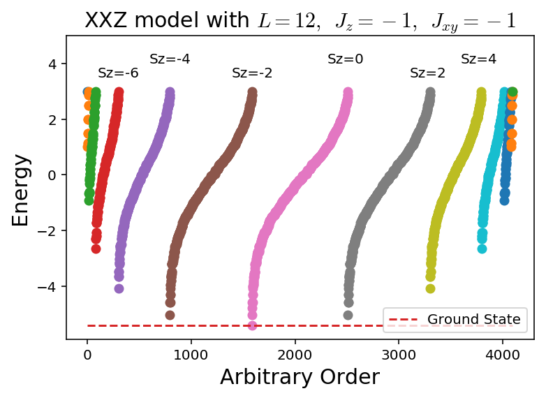
====
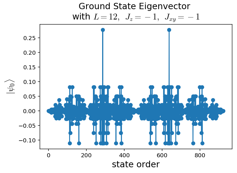
L = 12 basis size: 4096
The biggest states are:
|↓|↑|↓|↑|↓|↑|↓|↑|↓|↑|↓|↑|
|↑|↓|↑|↓|↑|↓|↑|↓|↑|↓|↑|↓|
CPU times: user 2.73 s, sys: 191 ms, total: 2.93 s
Wall time: 2.24 s
Notice how the maximal states of the ground state are the most antiferromagnetic states, but there is no difference to the model over the first and second one.
There’s also lower and lower energy, the lower total \(|S_z|\) is, which is expected as we want the least ferromagnetic configuration we can create.
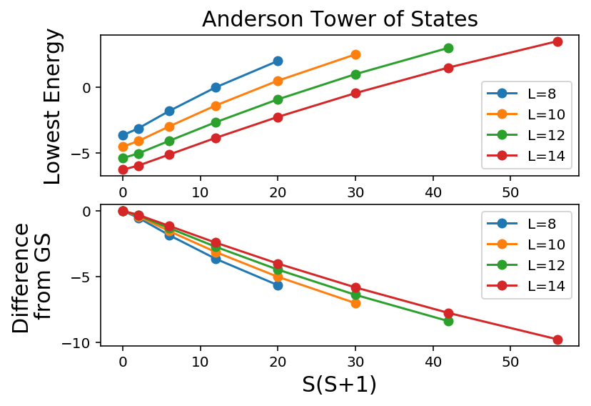
Anderson Tower of States
Secretly, in the thermodynamic limit there is sponanteous symmetry breaking with the antiferromagnetic ground state, along with gapless goldstone boson modes that come with it. Exact Diagonalization cannot see these as the system size is finite, however we can see the “hidden” effects of it.
Given an eigenstate from our computed spectrum, we’ll need to calculate the total spin expectation value \(\langle S^2\rangle\) or
\[S^2 =(S_1+\dots+S_L)^2= \sum_{i,j} S^{z}_iS^z_j + \frac{1}{2}(S^+_i S^-_{j} + S^-_i S^+_{j}))\]def calcTotalS(L,stateList,basisMap,eigvector):
'''Given an eigenvector, calculate <S^2>=S*(S+1)'''
totalS = 0
for i in range(len(eigvector)):
currState = stateList[i]
amp = eigvector[i]
for ix in range(L):
for jx in range(L):
if (currState>>ix & 1) == (currState>>jx & 1):
totalS += 0.25*amp**2 #Sz, 1/4 = 1/2*1/2
if ix == jx: totalS+= 0.5*amp**2
else:
totalS -=0.25*amp**2 #Sz -1/4 = +1/2 * -1/2
mask = 2**(ix)+2**jx
flipState = currState^mask #this flips the bits at i,j
idxFlip = basisMap[flipState]
totalS += 0.5*amp*eigvector[idxFlip]
return totalS
#unit tests
if np.abs(calcTotalS(2,[3],{3:0},[1]) - 1*(1+1)) > 1e-6:
raise ValueError("Bad <S^2>")
if np.abs(calcTotalS(2,[0],{0:0},[1]) - 1*(1+1)) > 1e-6:
raise ValueError("Bad <S^2>")
if np.abs(calcTotalS(2,[1,2],{1:0,2:1},[1/np.sqrt(2),-1/np.sqrt(2)]) - 0*(0+1)) > 1e-6:
raise ValueError("Bad <S^2>")
if np.abs(calcTotalS(2,[1,2],{1:0,2:1},[1/np.sqrt(2),1/np.sqrt(2)]) - 1*(1+1)) > 1e-6:
raise ValueError("Bad <S^2>")
%%time
Jxy = -1
Jz = -1
h = 0
minEList = []
minEList_goldstone = []
minSList = []
LList = [8,10,12,14]
for L in LList:
basisSzList = makeSzBasis(L)
SList = [] #this will hold all the S^2 values and what their energies are
EList = []
for sZ in range(len(basisSzList)//2+1):#exploit the Sz symmetry
SzList = basisSzList[sZ]
basisMap = {}
stateID = 0
#generate the ordering
for state in SzList:
basisMap[state] = stateID
stateID+=1
H = makeH(SzList,L,Jxy,Jz,h)
lam,v = np.linalg.eigh(H)
numStates = min(len(lam),10) #eigenvalues are sorted smallest to largest
EList = EList+list(lam[:numStates])
for i in range(0,numStates):
SList.append(np.round(calcTotalS(L,SzList,basisMap,v[:,i]),2))
SList,EList = zip(*sorted(zip(SList,EList))) #sort them by S^2
#now find all the S^2 values and determine the minimum
idx = 1
start = 0
end = 1
uniqueS = [SList[0]]
uniqueE = []
uniqueE_goldstone = []
while idx!=len(SList):
if uniqueS[-1] != SList[idx]:
end = idx+1
uniqueS.append(SList[idx])
ESort = sorted(EList[start:end])
uniqueE.append(ESort[0])
if len(ESort)>1:
uniqueE_goldstone.append(ESort[1])
else:
uniqueE_goldstone.append(ESort[0])
start=idx
idx+=1
ESort = sorted(EList[start:])
uniqueE.append(ESort[0])
if len(ESort)>1:
uniqueE_goldstone.append(ESort[1])
else:
uniqueE_goldstone.append(ESort[0])
minSList.append(uniqueS)
minEList.append(uniqueE)
minEList_goldstone.append(uniqueE_goldstone)
#plot!
plt.subplot(211)
for i in range(len(minEList)):
plt.plot(minSList[i],minEList[i],'-o',label="L="+str(LList[i]))
plt.legend()
plt.xlabel("S(S+1)",fontsize=15)
plt.ylabel("Lowest Energy",fontsize=15)
plt.title("Anderson Tower of States",fontsize=15)
plt.subplot(212)
for i in range(len(minEList)):
plt.plot(minSList[i],[minEList[i][0]-en for en in minEList[i]],'-o',label="L="+str(LList[i]))
plt.legend()
plt.xlabel("S(S+1)",fontsize=15)
plt.ylabel("Difference\nfrom GS",fontsize=15)
plt.show()
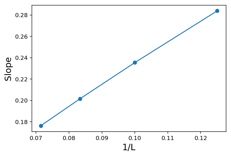
#plot the slopes
slopes = []
for i in range(len(minEList)):
slope, intercept, r_value, p_value, std_err = spst.linregress(minSList[i][1:],minEList[i][1:])
slopes.append(slope)
plt.plot([1/L for L in LList],slopes,'o-')
plt.xlabel("1/L",fontsize=15)
plt.ylabel("Slope",fontsize=15)
plt.show()
L = 8 basis size: 256
L = 10 basis size: 1024
L = 12 basis size: 4096
L = 14 basis size: 16384
CPU times: user 1min 18s, sys: 2.15 s, total: 1min 20s
Wall time: 1min 14s
What is going on? We see that the degenerate states that occur in the thermodynamic limit are slowly coming down. How fast are they coming down? \(1/L\), which is shown in the second plot.
#===============================================
%load_ext watermark
%watermark
2018-12-21T13:01:39-05:00

CPython 3.7.0
IPython 6.4.0

compiler   : Clang 9.0.0 (clang-900.0.39.2)
system     : Darwin
release    : 18.2.0
machine    : x86_64
processor  : i386
CPU cores  : 4
interpreter: 64bit